Stress and Losses Among Middle-Market Senior and Unitranche Loans: Introducing Cambridge Associates’ New Database
As part of our ongoing commitment to alternative credit, Cambridge Associates (CA) began compiling a database of credit stress and losses in one of the largest strategies within private credit, senior debt (i.e., direct lending). Our initial outreach in the United States and Europe yielded data from 11 senior debt funds tracking material document modifications (which we use as a proxy for credit stress, greater detail below) and loss rates in bilateral and clubbed middle-market lending. We expect this initial sample to grow as we add new managers and new vintages, and we are extremely grateful for the cooperation of the reporting funds and their pioneering involvement.
We expect to increase the number of reporting senior debt funds and to update our report annually with several goals in mind. First, we believe that this will help us make better decisions in building private credit and senior debt portfolios for our clients. Second, we believe that the stress and loss data demonstrate that senior debt funds can offer sound risk-adjusted returns for certain investors. By sharing these results, we hope to increase the acceptance of this asset class for appropriate investors. Finally, we believe that by collecting this data, we can provide some transparency into an opaque corner of the alternative credit market and address the concerns surrounding risk of loss in middle-market lending.
The current sample holds more than 2,700 loans amounting to $60 billion in original principal made between 2002 and 2017. We believe that the data show senior debt funds are adept at handling credit stress and minimizing losses over time. We will rely on our data to support our conclusions and will compare this asset class with broadly syndicated loans (BSLs) only selectively. Such a comparison is questionable because middle-market loan exposure is typically accessed through senior debt funds, which build portfolios muting the impact of individual losses (see the appendix for further discussion). BSL loss data, on the other hand, describe instrument level losses. Furthermore, the comparison is too difficult because the definitions of default and loss employed by credit ratings agencies when evaluating BSLs and senior debt funds are very different. Nevertheless, the wide acceptance of BSLs and the robust default and loss data warrant mention.
Our analysis of the data suggests that portfolios of middle-market senior and unitranche loans historically provided excellent downside protection for investors. The highest level of credit stress, as exhibited through material loan modifications, occurred with the 2007 vintage of loans, in which two of ten loans saw material modifications. Losses in the event of stress ranged by vintage from 0% to 64% of stressed credits.
Definitions and Methodology
Our Default Definition—Not Default, but Stress
Ratings agencies define default as a missed interest or principal payment, filing for protection under the prevailing bankruptcy code, or a distressed exchange of an instrument. We believe this definition of default is far too narrow to capture senior debt funds’ comparable credit problems because those funds will generally modify their credit documents to accommodate borrowers in distress. For example, it is highly unlikely that a middle-market borrower will surprise a senior debt fund with a missed payment. A CFO of a middle-market company failing to forewarn its only large lender of payment difficulty would probably be swiftly terminated. It is far more likely that the borrower will contact the lender, apprise it of difficulty, and ask the lender to permit the borrower to forego the cash interest payment for several periods and instead add it to the principal balance of the loan, a practice known as paying-in-kind, or PIKing. In this not uncommon scenario, the borrower would not default in the sense of the ratings agencies’ definition and would be fully compliant with an altered credit document, despite being unable to pay interest.
Furthermore, many middle-market companies have simple capital structures and small asset bases, making bankruptcy too expensive and protracted when compared to a negotiated outcome between the borrower and its only lender. In light of the frequency of bankruptcy filing as a path to default in the BSL market, 1 we suspected that strict adherence to the ratings agencies’ definition of default would understate credit stress in our sample.
Standard & Poor’s Leveraged Commentary and Data (LCD Comps) hints at these phenomena in its data set of BB/B-rated leveraged loans. Figure 1 shows cumulative default curves by tranche size and reveals that smaller tranches default at a far lower rate than larger tranches. We believe our explanation that smaller borrowers with fewer lenders tend to negotiate around payment defaults, bankruptcy, and distressed exchanges accounts for much, if not all, of this difference. (See the appendix for other explanations.)
FIGURE 1 CUMULATIVE DEFAULT CURVES BY TRANCHE SIZE
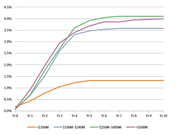
Source: Cambridge Associates LLC.
Recognizing the limited applicability of the ratings agency definition of default to the specifics of middle-market direct lending, CA broadened the definition of default to include: (1) all material modifications of loan documents; (2) PIKing not at the borrower’s option (i.e., excluding PIK toggle structures); and (3) cessation of accrual of interest and distressed covenant waivers. In general, material modification refers to the “sacred rights” of credit documents—to wit, any term or condition that affects yield and which requires unanimous lender approval (e.g., term, interest rate, amortization, commitment, etc.). CA’s database, therefore, does not track actual defaults as material loan modification, which we interpret as evidence of general credit stress in a portfolio. Put another way, lack of material modifications in loan documents usually, but not always, implies a healthy borrower that can make its interest and principle payments in a timely manner and in compliance with all existing covenants. Naturally, the rate of stress in our sample will exceed default rates observed in the BSL market, and this has significant implications for recovery analysis (see the appendix). Nevertheless, we believe it offers a more searching calculus to underpin prudent capital allocation. We will refer to modifications and credit stress interchangeably.
However, we recognize that our approach also has drawbacks. Just as the ratings agency definition may render false negatives, our definition of stress may yield false positives: instances qualifying as stress where in fact none or very little exist. For example, the unexpected opportunity to purchase a competitor or a new factory may require both a capital expenditure covenant waiver and an amortization holiday. Similarly, a borrower slated for sale just prior to a loan’s impending maturity may see the sales process stalled through no fault of its own, requiring an immediate extension of the maturity pending resolution of the obstacles to the sale. These events would require material modifications to a credit document that would be caught in our definition of credit stress, when in fact the borrower may be performing to plan or better.
Understanding that stress can mean almost anything from outright business failure to virtually immaterial documentary changes is vital to reading our analysis. The broad definition is, therefore, perhaps most helpful in its counterfactual: loans experiencing no reported credit stress very likely performed to or above plan at underwriting. When reading the stress rate analysis below, the reader should consider this alternate perspective.
Loss Definition—Very Basic
When comparing recoveries, we used publicly available information from Moody’s because they calculate recoveries based on trading price and recoveries based on ultimate recovery. The former is calculated as the discounted (at the coupon rate) trading recovery price as a percentage of the original par value. The latter seeks to identify actual recoveries and is “the value creditors realize at the resolution of a default event. For example, for issuers filing for bankruptcy, the ultimate recovery is the present value of the cash or securities that creditors actually receive when the issuer exits bankruptcy, typically one to two years following the initial default date.” 2
CA recognizes that replicating this level of detail for middle-market loans is impracticable. As a result, we gathered data reflecting the total amount of principal collected excluding interest and fees. CA further recognizes that senior debt funds calculate losses and recoveries differently and sought to implement a standard method with minimal scope for manipulation. Our loss and recovery rates, therefore, exclude any recovery from interest and fees.
Another difference between our method and that of the ratings agencies is their focus on individual instrument recoveries. While this is theoretically the best way to aggregate recovery data, we believe that collecting this level of data from senior debt funds would prove onerous. As a result, we calculate losses and recoveries on aggregate vintages, generating a directionally accurate average. Vintage losses are calculated by dividing the par value of losses incurred by a vintage by the aggregate reported par value of that vintage. 3 Recovery rates are calculated by subtracting that rate from one.
We hope to provide an estimated range of recoveries for middle-market loans and to compare them to the information provided by CRAs compare the relative risk of loss for BSLs and middle-market loans.
Caveats and Methodology
Importantly, CA did not audit the data provided and relies solely on what was reported by cooperating senior debt funds. As a result, we rely on the honesty and forthrightness of participating senior debt funds. Our interaction with these lenders, their detailed questions, desire for elaboration, and specification of our methods and criteria lead us to conclude that they are trustworthy partners in this exercise.
As noted, we received data on first-lien senior loans, including unitranche loans, from 11 senior debt funds totaling 2,728 loans with $61.7 billion in aggregate par value and average original par value of $22.6 million. Loans were categorized by origination year and then tracked by stress year and loss year. Our data set shows aggregate loans issued in each year from 2002 to 2017 and aggregate stressed loans and losses of each vintage. CA can therefore report, for example, total loans issued by number and par value in 2002 (the 2002 “vintage”) and total number and par amount of stressed loans and losses of that vintage in years 2002 through 2018.
When calculating credit stress, we rely on loan count, and when calculating losses, we rely on value. We believe that this reflects the maxim that borrowers default and instruments recover. In addition, this approach comports with that of LCD Comps, which offers a very comparable methodology and data set.
While we believe that our total sample size of loans is robust, we recognize that it represents a small sample of the entire universe of middle-market loans. Moreover, we recognize that the reporting funds create two biases. First, some funds that declined to participate may fear that their performance is poor relative to peers. If that fear is valid, then their absence improves the overall data set. (We do not suggest that non-participating senior debt funds all have inferior modification and loss experience—merely that the possibility exists.) Second, reporting funds in existence prior to 2008 create a survivorship bias. In other words, we do not have data from those funds that did not survive the global financial crisis (GFC).
Findings, Results, and Conclusions
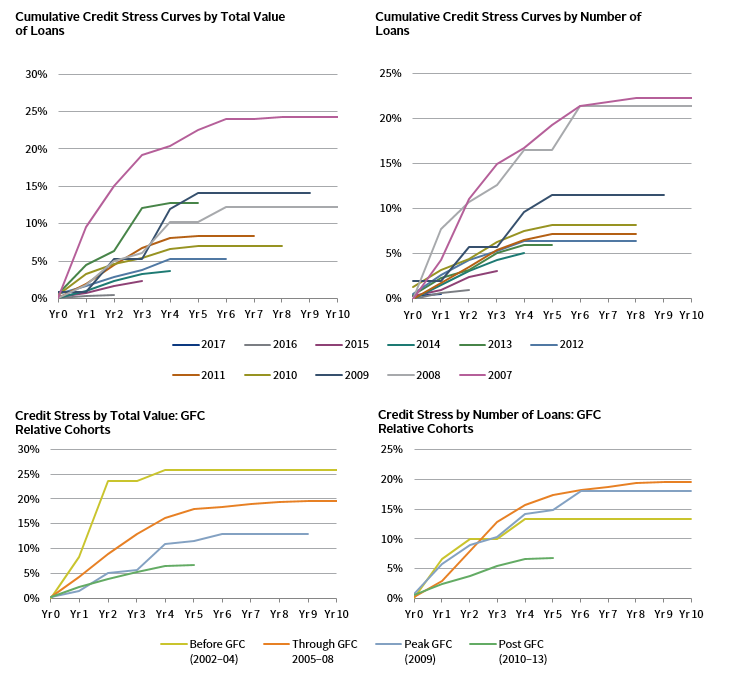
In Figure 2, our findings and sample size are broken out by vintage. We analyzed the data by vintage and across all vintages on an annual and cumulative basis. We also divided the data into cohorts by vintage depending on the likelihood that the loans would have lasted through the GFC. 4
FIGURE 2 RESULTS BY VINTAGE YEAR
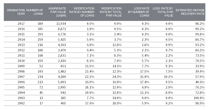
Source: Cambridge Associates LLC.
Note: The Estimated Vintage Recovery Rate is calculated as 1 – (Loss Rate by Value/Stress Rate by Value).
Credit Stress Analysis
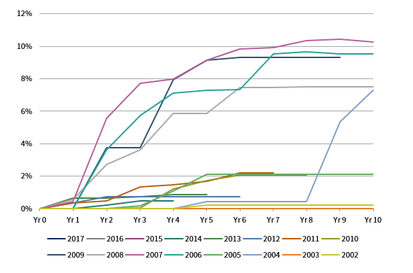
Figure 3 shows the cumulative credit stress rate for all of the loans in our sample. In generating this curve, we employed the same arithmetic approach as LCD Comps in generating the curves presented above: the cumulative observations of stress (by borrower count) for each year are divided by 2,728, the total number of loans made from 2002 to 2017. Recognizing that the entire sample includes loans from 2013 to 2017, which have not seasoned, we show a curve with vintages from 2002 to 2012.
FIGURE 3 CAMBRIDGE ASSOCIATES CUMULATIVE “CREDIT STRESS” RATE
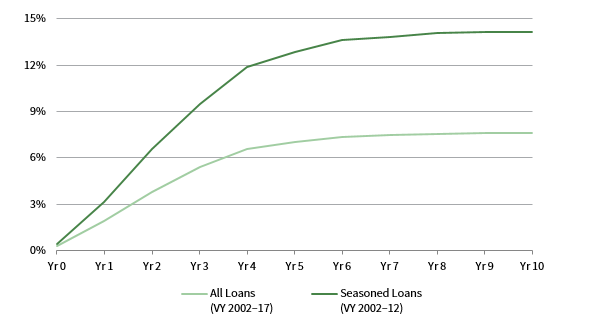
Source: Cambridge Associates LLC.
The curve clearly shows that the incidence of stress is far higher in our sample than the highest default of 4% in the LCD Comps sample used to generate Figure 1. We hesitate to compare actual ratings agency default incidence to our incidence of stress because our approach should capture everything from a benign documentation change described above all the way to liquidation.
We believe the best reading of this curve concludes that approximately 85% of total borrowers in the seasoned cohort did not seek and were not granted material loan modifications by year 10 and therefore experienced little to no credit stress.
Within that cohort, the incidence of material modifications ranged from 6.4% (2012) to 22.2% (2007). By comparison, LCD Comps reports default rates ranging from 0.7% (2009) to 12.0% (2007). As expected, the implied rate of credit stress exceeds default rates. However, we believe that the data suggest that credit stress, broadly defined by material modifications, occurs less frequently than many may believe, affecting one in five borrowers at the height of the GFC (i.e., the 2007 vintage). The appendix further breaks out each individual vintage, as well as cohorts of vintages relative to their position before, during, and after the GFC.
Measuring Losses: The Challenge of Vintage Data
We recognize that stress rates do not answer the burning question of how much a senior debt fund can expect to lose. We note the aggregate losses in Figure 2 and the par value weighted loss curves are presented below. Figure 2 shows that recovery rates in the event of stress can range from 100% to as little as 34% (in the 2009 vintage) and that vintages have historically lost between 0% and 10% of their aggregate principal balance. We further note that these loss rates were not experienced by particular fund vehicles. 5 In the case of 2009, 14.1% of the total portfolio encountered stress and 9.3% of the total portfolio was lost. Our loss-given-stress calculation divides the loss rate by the stress rate to show that approximately two-thirds of the value of stressed (or modified) loans were lost.
The stress rate here is critical when considering loss given stress. Two of the three worst recovering vintages, 2009 and 2010, raise practitioners’ eyebrows because these vintages should have offered the best opportunities to lend, yet their loss-given stress levels are very high, and their implied recoveries are very low. However, Figure 4 shows the relationship between stress and loss is critical when deriving loss estimates. For example, in 2010 a greater percentage of modified loans incurred losses, even if absolute losses were low. This may be attributable to the fact that fewer loans made in 2010 struggled at all (suggesting a healthy credit environment), but those that did struggled mightily, with losses of $109 million on $168 million of modified loan value.
FIGURE 4 MODIFICATION RATES AND LOSS RATES OVER TIME
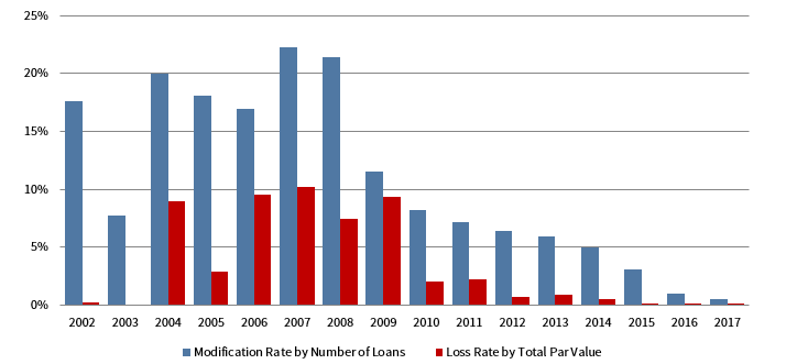
Source: Cambridge Associates LLC.
A comparison of 2009 and 2004 sheds further light on the importance of the relationship between modifications and losses. For 2009, our sample shows 52 loans made with six modifications (total value of $120 million) generating a stress ratio of 11.5%. Four of those loans, however, incurred losses of $79 million, or 9.3% of total par value. By comparison, 2004 saw 45 loans made with nine incidents of stress, a rate of 20%, almost double that of 2009. Losses in the 2004 vintage were 8.9%, roughly in line with 2009. The big disparity between stress rates generates a very large difference in loss-given stress.
There are a couple possible explanations for this phenomenon. For 2009, one may simply be sample size. The 2009 vintage had one of the lowest loan counts in the sample, exposing it to greater variation of outcomes. Another may be that some loans may have been committed to later in 2008 and so were made before the full force of the GFC impacted borrowers. The 2010 phenomenon is more difficult to explain. The majority of losses in this vintage were actually incurred in 2017 ($59 million of $109 million), more than six years after origination. Loans tend to sour in the first two to three years after origination. It is possible that this vintage may have been overly exposed to sectors that deteriorated later and for reasons unrelated to the GFC (e.g., energy, retail, etc.). We would, therefore, suggest that investors focus on gross losses rather than losses as a percentage of stressed assets.
Furthermore, our database offers certain insights into losses that can help investors form an opinion about the risk of loss in middle-market loans. We frequently hear concerns that middle-market companies can just “go away,” leaving lenders with little or no recovery. Our data hint at this risk. At the same time, there is more direct evidence of robust recoveries. For example, of the three vintages reporting one loan loss, all recovered more than 98% of principal. While we realize that middle-market companies, not unlike their larger peers, can “just go away,” we resist the commonly held belief that their disappearance is the norm.
Insights from Vintages
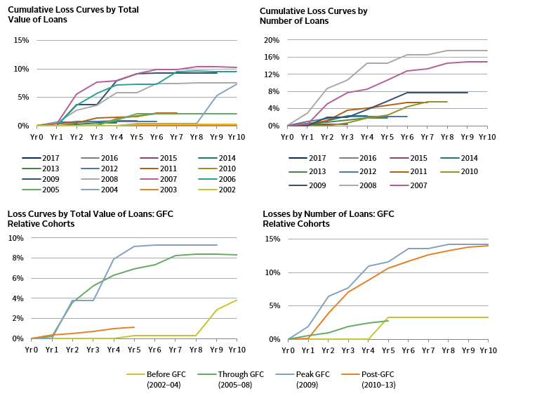
Building on our previous work “Origination Year Defaults: A Canary in the Credit Coal Mine?,” which demonstrated the importance of vintage even among identically rated loans, we broke out loss curves by origination year for our senior debt fund loans. As expected, the vintages with the highest cumulative loss rates are 2006 through 2009 because they are clustered around the GFC. The 2004 vintage is particularly interesting, as losses spiked in 2012 and 2013 to 2008 peak levels, which is likely related to small sample size (Figure 5).
FIGURE 5 CUMULATIVE LOSS CURVES BY TOTAL VALUE OF LOANS
Source: Cambridge Associates LLC.
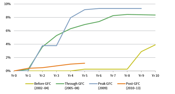
Figure 6 categorizes all the vintages into four cohorts: (1) before the GFC, 2002–2004, whose loans likely seasoned before 2008; (2) through the GFC, 2005–2008, whose loans were made just prior to the GFC and therefore were serviced during the GFC; (3) during the GFC, 2009, which were made when the crisis was at its worst; and (4) post-GFC, 2010–2013. CA recognizes that some of these loans may still be outstanding and could still incur losses.
FIGURE 6 LOSS CURVES BY TOTAL VALUE OF LOANS: GFC RELATIVE COHORTS
Source: Cambridge Associates LLC.
Model Portfolio Creation and Simulation
Finally, CA attempted to create a model portfolio of loans in our data set to simulate the actual year-to-year performance (Figure 7). We did this by chronologically adding each reported annual par value to the net sum of the previous year’s existing outstanding loan balance, less actual losses in that year, and estimated repayment. Annual losses rose to approximately 4% in the teeth of the GFC and then declined as old loans repaid and were replaced by new, unseasoned, performing loans.
The simulation in Figure 7 does not guarantee performance for senior debt funds and is based on assumptions that may be faulty. However, it helps to frame an analysis of senior debt fund performance and provides a superior analytical lens compared to individual loan losses.
FIGURE 7 SIMULATED LOSS RATE
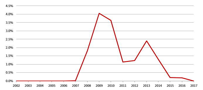
Source: Cambridge Associates LLC.
Finally, we formulated a hypothetical “worst case” scenario senior debt fund with a five-year investment period from 2005 to 2009, the years leading into and through the GFC. We further assumed that the losses happened immediately, generating no interest or amortization to cover losses and forcing the “fund” to rely on the performing loans to cover losses and generate returns.
Figure 8 suggests that despite lending into and through the GFC at a small spread over LIBOR, a senior debt fund would very likely not have lost LP capital at the portfolio level (as denoted by the multiples of less than 1.0x). These loans would have probably generated a safe, if unspectacular, return on invested capital of approximately 1.1x at the portfolio level. Moreover, if these loans were made at the average prevailing one-month LIBOR rate with no spread (i.e., L+0.0% coupon), the performing loans’ interest could have compensated for the losses incurred in 2005, 2006, and 2007 (when average one-month LIBOR calculated on a daily basis was 3.3%, 4.9%, and 5.1%, respectively), and those vintages could also have compensated the portfolio for losses incurred in 2008 and 2009 (when average one-month LIBOR calculated on a daily basis was 2.6% and 0.3%, respectively). Our analysis does not forecast or guarantee performance of senior debt funds through the next credit cycle. Instead, it is meant to strongly suggest that LPs would run a very low risk of losing capital invested exclusively through one of the worst economic downturns of the last century. 6
FIGURE 8 PERFORMANCE OF SENIOR DEBT FUNDS THROUGHOUT THE GFC
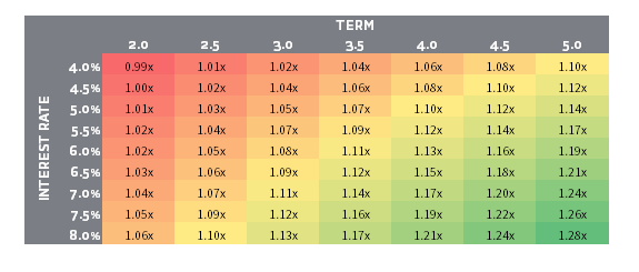
Source: Cambridge Associates LLC.
Notes: Excludes management fees and carry and impact of fund level leverage. Average one-month LIBOR calculated daily from 2005–09 averaged 3.25%.
Conclusion
The analysis confirms our belief that senior debt funds have historically demonstrated resilience in the face of economic stress and have offered LPs a low volatility, yield-generating investment opportunity. We believe that many of these attributes will persist. However, we also recognize that deterioration in loan terms, higher leverage, and other pernicious developments in the middle market will erode that historic resilience. Nevertheless, there are some senior debt fund managers that can negotiate the treacherous currents within the middle market and could emerge with performance similar, if not superior, to historic observations. ■
Appendix
LCD Default Curves: Alternative Explanations
We posit that smaller tranche sizes exhibit lower default incidence because the loans are made by smaller groups of lenders that can alter documents to accommodate borrowers and thereby avoid defaults. Another plausible explanation for this profound difference could simply be that the borrowers of tranches less than $100 million are as large as those borrowing more, but are less levered and therefore less likely to default. LCD data do not appear to disclose borrower size or leverage level. Based on experience and discussions with senior debt fund managers, we believe that our explanation is more likely.
APPENDIX FIGURE 1 CUMULATIVE DEFAULT CURVES BY TRANCHE SIZE
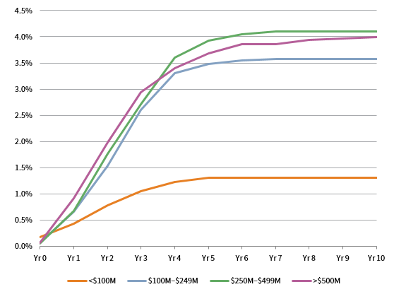
Source: Cambridge Associates LLC.
Curves Broken Out by CA Data Set Vintage
As with larger loans, vintage can play an important role. The curves suggest that through the GFC, 80% of loans by number of loans and 75% of loans by total value of loans exhibited little to no financial stress.
We repeat the caveat that while we view our sample size of loans in terms of number and outstanding principal as generally robust, we recognize that the reporting universe of 11 senior debt funds is small relative to the outstanding population. We also realize that the majority of reporting funds did not lend through the GFC.
APPENDIX FIGURE 2 CREDIT STRESS
Source: Cambridge Associates LLC.
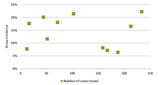
Sample Size
Concerns raised over distortions wrought by small sample sizes do not appear to plague our data. The figure below shows that instances of stress do not correlate to the number of issued loans.
APPENDIX FIGURE 3 REPORTED STRESS RATES AND NUMBER OF LOANS ISSUED
Source: Cambridge Associates LLC.
While we include losses by number of loans, we suggest focusing on losses by value. The data underscore the importance of vintage in assessing loss probability, but also show that staggered vintage deployment mitigates losses.
What does it mean for recoveries when stress exceeds defaults?
The cornerstone calculation for any credit investor is the product of the probability of default (PD) and the loss-given default (LGD), which yields expected loss (EL).
PD X LGD = EL
In our sample, we use “loss-given stress” as a proxy for LGD, but in practice it would be very difficult for a loan to lose principal without suffering a default as defined by the ratings agencies in the BSL market.
Our analysis notes that the probability of credit stress (PCS) exceeds PD observed in the BSL market and suggests that BSL EL (ELBSL) is broadly in line with middle-market EL (ELMM).
PDBSL X LGDBSL ~ PCS X LGSMM
Expected losses should not change. However, if we remove the parts of credit stress that fall short of actual defaults, then PCS should decline in the equation above. For the identity to survive, LGDMM must increase.
APPENDIX FIGURE 4 LOSSES
Source: Cambridge Associates LLC.
Simulated Losses
The simulated loss rate in Figure 7 may provoke skepticism. Senior debt is a relatively new asset class geared toward financing borrowers that are too small to tap the capital markets. Investors may believe that inability is rooted in poor creditworthiness, when in fact, it is more likely the result of investment banks’ affinity for the fees generated by larger borrowers. One way to “sanity” check the simulation presented above is to find entities that resemble senior debt funds’ strategies. The most obvious analogy is the business development corporation (BDC). Many senior debt funds have affiliated BDCs. However, based on market research, many BDCs tend to house assets that would be considered riskier than the senior and unitranche loans analyzed in this report.
APPENDIX FIGURE 5 CHARGE OFF RATE: COMMERCIAL & INDUSTRIAL LOANS (US)
January 1, 1985 – January 1, 2019 • Percent
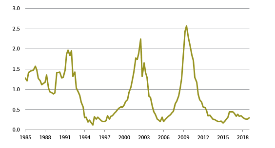
Source: Federal Reserve Bank of St. Louis.
Commercial banks offer a more comparable group of lenders with their focus on senior corporate loans. In fact, many senior debt funds identify bank withdrawal from core markets as the genesis of their opportunity set. US regulators capture loan provisioning rates for domestic commercial banks, and their trends and levels resemble the contours of our simulation, particularly at the height of the crisis.
Footnotes
- According to Moody’s Investors Service, 19 of 61 defaults in 2018 and 34 of 91 in 2017 came as a result of bankruptcy filing.
- Defaults will rise modestly in 2019 amid higher volatility, according to Moody’s Annual Default Study. See Moody’s Investors Service, “Annual Default Study: Defaults Will Rise Modestly in 2019 Amid Higher Volatility,” February 2019.
- Based on the identity: Recovery Rate = 1 – Expected Loss where Expected Loss = Probability of Default * Loss Given Default.
- Vintage is important not only to middle-market loans but also to BSLs. In our previous work, we demonstrated that cumulative defaults by vintage ranged from less than 1% to almost 20% for BB- and B-rated loans tracked by LCD Comps from 1995 to 2017.
- We asked senior debt funds only for senior and unitranche loans that did not qualify as BSLs. As a result, fund vehicles may have held the loans in our database as well as BSLs, second-lien loans, preferred equity, etc. and would therefore experience loss incidence at the fund level different from our sample of loans.
- A portfolio of BSLs would exhibit similar characteristics. The point of this analysis is not to argue that a portfolio of middle-market loans offers superior protection from principal loss, but rather to address concerns over losses and defaults at the fund level and to point out that middle-market loans can generate adequate interest coverage to cover losses, a critical attribute of credit spread investing.
About Cambridge Associates
Cambridge Associates is a global investment firm with 50+ years of institutional investing experience. The firm aims to help pension plans, endowments & foundations, healthcare systems, and private clients achieve their investment goals and maximize their impact on the world. Cambridge Associates delivers a range of services, including outsourced CIO, non-discretionary portfolio management, staff extension and alternative asset class mandates. Contact us today.