Quantitative Tightening Raises the Risks for Markets


With inflation running at multi-decade highs, monetary policymakers are united in one of the most aggressive tightening campaigns in decades. Most central banks have already significantly increased policy rates this year, and some are unwinding their massive balance sheets, also known as quantitative tightening (QT).
From what we know about QT, we expect it to tighten liquidity conditions, put upward pressure on interest rates, and possibly lower equity multiples, all else equal. However, there is considerable uncertainty about the magnitude of its impact. Given this uncertainty, we review what is known about the current state of central banks’ balance sheets and their operations, discuss some known uncertainties of QT’s impact on financial markets, and consider QT in the context of the current market environment.
With QT just now ramping up, the risk it poses to financial markets appears low. Yet, adding QT to what is an already difficult and volatile market environment may worsen market conditions, increasing the risk that “something breaks” from overtightening. While we caution against any significant change to portfolio allocations in response to QT, the balance of risks suggests now is an appropriate time to strengthen stress tests of portfolio liquidity. The goal is to ensure portfolios are not only well diversified to handle a variety of market outcomes, but are positioned to take advantage of opportunities that may arise during periods of market stress.
What We “Know” About Central Bank Balance Sheets and Their Operations
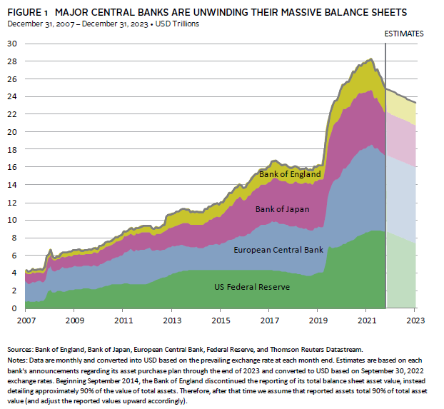
As part of their tightening efforts, central banks are discussing, or have already started, rapidly unwinding their massive balance sheets. Most notably, the Federal Reserve stopped reinvesting all maturing debt held on its balance sheet in June at an initial cap of $47.5 billion per month, increasing to $95 billion per month in September. The rapid pace of QT will significantly reduce the size of global central banks’ balance sheets, with the Fed’s planned QT alone reducing the total cumulative balance sheet assets of the world’s four major central banks by roughly $1.6 trillion by the end of 2023 (Figure 1).
The effects of this reduction in central bank balance sheets are well understood from a mechanical standpoint, where QT reverses many of the impacts of quantitative easing (QE). For example, as the Fed shrinks its balance sheet, it removes the liquid bank reserves that were added during QE, while the Treasury issues new government securities to finance the maturing bonds the Fed purchased during QE. Thus, whereas QE seeks to ease financial conditions, QT tightens them by removing liquidity from the banking system and increasing the supply of duration for the private sector to absorb, putting upward pressure on interest rates.
However, while the mechanics of QT are understood, there is considerable uncertainty about the degree to which it will tighten financial conditions above and beyond rate hikes. Much of this uncertainty stems from a lack of experience with QT, which raises questions about how much QT the market can handle and, as a result, its overall impact on financial markets.
Known Unknown #1: How Much QT is Too Much?
QT is not a permanent operation. At a certain point, aggregate bank reserves and central bank balance sheets will shrink to more “normal levels.” However, quantifying this level remains a large uncertainty, and there is a risk of overtightening if central banks remove “too many” reserves from the banking system.
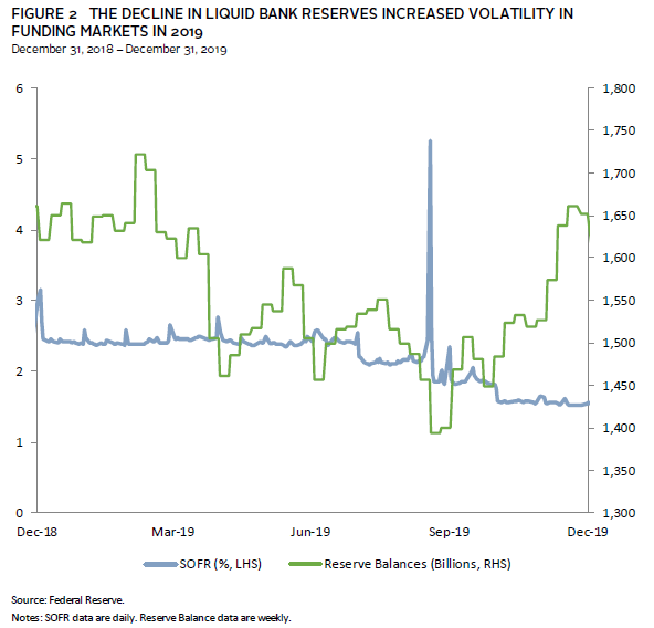
The Fed’s experience with QT between 2017 and 2019 highlights how it can disrupt markets (Figure 2). Fed analysis at the time estimated the optimal level of bank reserves as between $700 billion and $900 billion. However, key funding markets experienced considerable stress in September 2019 when aggregate reserves were still at $1.5 trillion. During this episode, larger demands for liquidity caused banks to pull back from short-term funding markets and hoard reserves. Eventually, the Fed intervened to calm markets through repo operations and, importantly, by resuming asset purchases.
To be sure, global central banks may be far off from overtightening. Reserve balances have declined by roughly $1 trillion already this year, but they remain comfortably above analysts’ estimates of the minimum level of reserves of between $2.0 trillion and $2.5 trillion. Additionally, repo rates in the United States are trading around and, at times, below the lower bound of the Fed’s policy rate—a sign there is currently still ample liquidity in the banking system. As liquidity becomes constrained, we would expect short-term repo rates to reach and potentially spike above the upper bound of the Fed’s policy rates, as they did between 2017 and 2019.
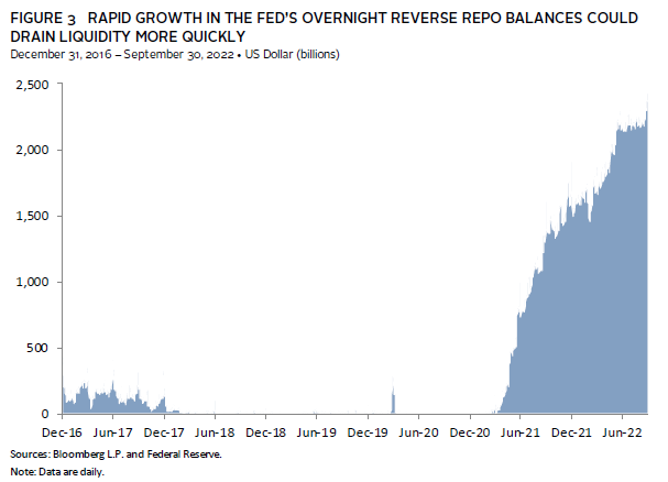
However, the faster pace of QT combined with a growth in the Fed’s Overnight Reverse Repo (ON RRP) balances could accelerate the decline in liquidity past what the Fed originally anticipated. The ON RRP essentially acts as a release valve for the excess liquidity created from QE. ON RRP balances have continued to grow despite QT’s start, even reaching all-time highs as recently as September 30 (Figure 3). Should this continue, reserve balances will be drained even further from the banking system, with an “overtightening” potentially occurring more quickly than originally anticipated.
Important guardrails have been put in place by the Fed to help manage stress in funding markets, such as its Standing Repo Facility, but market stressors seldom take identical forms. Thus, while the QT between 2017 and 2019 ended in a blow-up in short-term funding markets, today’s QT could have impacts elsewhere in the financial system, regardless of where liquidity shortages originate. This could include foreign exchange, commodities markets, or even sovereign stresses abroad, such as those recently experienced in the United Kingdom. Overall, QT makes such instances more precarious as less liquidity is available to be distributed system-wide to areas experiencing stress.
Known Unknown #2: QT’s Impact on Rates and the Yield Curve
Similarly, while most analysts agree QT likely puts upward pressure on interest rates, there is significant uncertainty about the magnitude of these effects, and, in practice, this relationship is less clear.
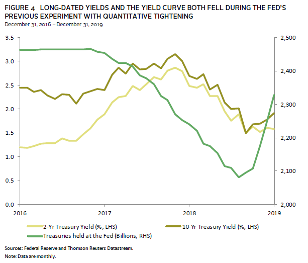
To understand this uncertainty, one need only look at the wide range of estimates produced by studies attempting to equate QT to rate hikes. 1 While empirical results vary widely, studies mostly agree that QT increases both interest rates and the yield curve. However, between 2017 and 2019, while US Treasury yields initially increased during QT, they ultimately fell, with ten-year yields and the yield curve declining over the full period (Figure 4).
This is likely because there are several factors that drove interest rates, which overwhelmed any impact from QT. This is especially true of yields further out the curve. As we look ahead, there are factors, such as the Treasury’s issuance plans, which confirm QT may only put modest upward pressure on the yield curve, all else equal.
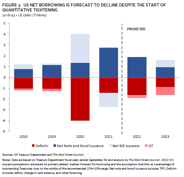
The Treasury will need to issue roughly $1.8 trillion new Treasury securities between 2022 and 2024 to replace the maturing bonds rolling off the Fed’s balance sheet, which is a much larger injection of duration for the private sector to absorb than between 2017 and 2019. However, the Treasury’s borrowing needs have declined sharply with the US federal budget deficit projected to decline. Additionally, the Treasury is considering operations to smooth QT, including issuing more T-bills initially. In fact, net Treasury notes and bonds issuance are forecast to decline in both fiscal year 2022 and 2023, according to analysis conducted by the Wall Street Journal (Figure 5).
Any change in yields further out the curve is also subject to many other factors, such as private sector demand for duration, which has waned this year amid concerns about high inflation and monetary tightening. Higher yields may attract more demand. However, it is likely that price sensitive (and levered) buyers will increasingly become the marginal buyers of Treasuries, suggesting the impact of QT on bond yields could grow over time, as such purchases tend to be more sensitive to macroeconomic outcomes and increasingly rely on short-term funding markets.
Known Unknown #3: Does QT Make Risk Assets Riskier?
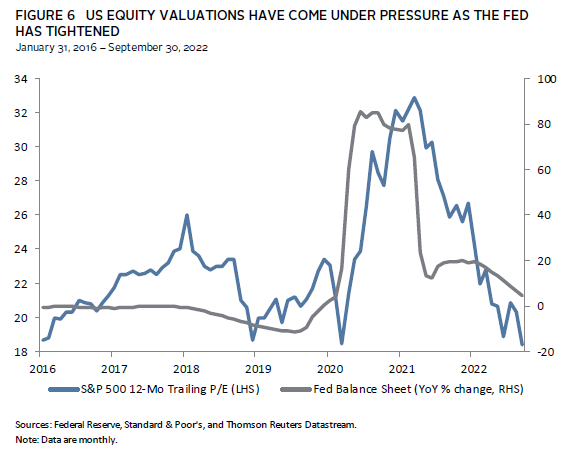
QT’s impact on interest rates will ultimately determine its impact on risk assets. Though the theory has its uncertainties, QE/QT impacts equity markets primarily through the “portfolio rebalancing effect,” as investors move out the risk curve when term premiums on yields further out the curve are condensed, and vice versa. This is evidenced in part by the drastic rise in US equity multiples during QE and subsequent decline this year (Figure 6).
While our limited experience with QT prevents us from relying too much on history to inform how equities might behave this time around, the Fed’s previous experiment with QT does provide some guidance. Between 2017 and 2019, US equity multiples contracted by nearly 30% peak-to-trough and equity volatility increased. It is important to note that the Fed also raised its Fed funds target range by 175 basis points (bps) over this period, though the 6% decline in the S&P 500 Index in August 2019 and 4% sell-off in September 2019 are largely attributed to stress in funding markets caused by QT, the latter of which may have been worse if the Fed did not intervene to stabilize markets.
Correlation is not causation, but it is hard to deny that risk assets have become more sensitive to monetary policy more recently. The correlation between trailing 12-month price-earnings (P/E) multiples for US equities and ten-year real yields was slightly positive prior to 2008. Since then, however, the correlation is -0.48. Today, a significant amount of tightening has already been priced into both equity and fixed income markets. Ten-year real yields in the United States have increased 272 bps so far this year and the S&P 500 Index has fallen 25% peak-to-trough, with the trailing P/E ratio contracting 31%. Therefore, any further impact from QT may be limited, at least initially, given the scale of the correction to-date.
QT in a Difficult and Volatile Market Environment
These uncertainties make it difficult to estimate the impact of QT on financial markets even under relatively “normal” market conditions. Though, it likely raises the risks for markets, all else equal. This may be even more true today, considering the added risk of introducing something as highly uncertain as QT to an already difficult and volatile environment.
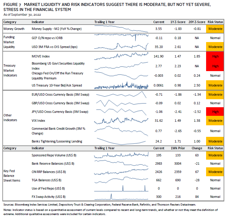
Today is a much different environment than the first bout of QT between 2017 and 2019. Inflation is at multi-decade highs, monetary policymakers are aggressively tightening policy, recession risk is rising, and financial markets are dealing with a wide variety of exogenous risk factors, such as the lingering effects of COVID-19, the war in Ukraine, and an energy crisis in Europe. We expect the addition of QT onto all these factors to add to market volatility. Currently, market risk and liquidity indicators are showing moderate stresses, particularly in Treasury markets, given the rapid pace of rate hikes this year (Figure 7). We expect QT will contribute to poor liquidity conditions next year. If those conditions become so poor that they risk financial stability, central banks may be forced to prioritize relieving short-term pressures over fighting inflation. To some extent, this is what happened with the Bank of England last month.
While we see risks on the horizon, we caution against any significant change to portfolio allocations in response to QT or other potential tail risks. Central banks may have a higher threshold for market stress in the current environment, which could increase volatility for safe assets and risk assets alike. However, we ultimately expect them to respond to severe bouts of financial market stress, at which point financial assets may rebound sharply. As such, now is an appropriate time to strengthen stress tests of portfolio liquidity. This will help ensure portfolios are not only well diversified to handle a variety of market outcomes but are able to take advantage of opportunities that may arise during periods of market stress.
Figure 7 Notes
M2 data are as of 8/31/2022. Bloomberg US Government Securities Liquidity Index data are as of 9/16/22. Banks Tightening/Loosing Lending data are as of 6/30/2022. Bank Lending Standards data are quarterly. Cross Currency Basis data are monthly. M2 Money Supply, BBG US Government Liquidity, Chicago Fed On-Off 10-Yr Liquidity Premium, Commercial Bank Credit Growth, Bank Reserves, TGA Balance, and FX Swap Activity Data are weekly. GCF Repo-IORB, 3M FRA-OIS Spread, Sponsored Repo Volume, Move Index, 10-Yr Bid-Ask Spread, VIX, ON RRP Balance, and Use of Fed Repo data are daily.
GCF O/N vs IORB
GCF O/N vs IORB reflects the overnight general collateral financing repurchase rate on Treasuries (GCF O/N) less the interest rate of Federal Reserve Bank balances (IORB).
3M FRA vs OIS Spread
3M FRA vs OIS Spread reflects the forward rate agreement (FRA) less the overnight index swap (OIS). FRA represents the interbank lending rate and OIS represents the effective fed funds rate where a higher spread indicates elevated funding stress.
MOVE Index
MOVE Index reflects volatility in the US Treasury market through US Treasury option pricing at various maturities.
ON RRP Balances
ON RRP Balances represents overnight reverse repurchase agreements at the Federal Reserve.
TGA Balances
TGA Balances represents the Treasury General Account balances, which are the primary operational account of the US Treasury at the Federal Reserve.
Index Disclosures
Bloomberg US Government Securities Liquidity Index
Bloomberg US Government Securities Liquidity Index is a gauge of deviations in yields from a fair-value model.
S&P 500
The S&P 500 gauges large-cap US equities. The index includes 500 leading companies and captures approximately 80% coverage of available market capitalization.
Footnotes
TJ Scavone - T.J. is a Senior Investment Director in the Capital Markets Research Group at Cambridge Associates.
About Cambridge Associates
Cambridge Associates is a global investment firm with 50+ years of institutional investing experience. The firm aims to help pension plans, endowments & foundations, healthcare systems, and private clients achieve their investment goals and maximize their impact on the world. Cambridge Associates delivers a range of services, including outsourced CIO, non-discretionary portfolio management, staff extension and alternative asset class mandates. Contact us today.