A Framework for Benchmarking Private Investments

Executive Summary
- Private investments often play an important role in an investor’s portfolio, yet the inconsistent methodologies typically used to evaluate private investment performance and public market performance result in a lack of understanding about true relative performance.
- The two most common measures of investment performance—time-weighted returns (TWRs) and money-weighted returns, typically an internal rate of return (IRR)—differ in meaningful ways. An IRR is a superior indicator of ultimate performance because it looks holistically at the time horizon of interest and considers all cash flows. Unlike the compounded TWR, an IRR captures the impact of managers’ investment decisions, including when to call and return capital, when to exit, etc. Nonetheless, IRRs are not perfect measures and investors should keep in mind issues associated with the IRR calculation, including the reinvestment rate assumption and the fact that the IRR can be managed in certain circumstances. To put IRRs in context, we recommend always reviewing IRRs alongside cash-on-cash multiples like distributed to paid-in capital and total value to paid-in capital.
- Private investment funds and corresponding benchmarks require a surprisingly long period of time before they provide any indication of ultimate performance. On average, a fund needs about six years to “settle” into its final quartile ranking versus peers. Funds can shift significantly among quartiles, with 80% to 90% of funds landing in at least three different quartiles through the course of their lives. Based on this analysis, we believe that drawing any conclusions about a manager’s performance earlier than five to six years into a fund’s lifecycle can lead to incorrect conclusions and poor selection of follow-on funds. Given the staggered commitment approach typical of private portfolios, this analysis implies that investors should not attempt to derive much meaning from private portfolio returns and benchmark comparisons until the program is at least eight years old.
- The lack of a single “right” measure for private investment performance has led to inconsistent approaches across the industry and difficulty decomposing the various drivers of performance. We have developed a framework that seeks to address this problem by measuring success across a series of key metrics and leveraging a set of tools that can be applied in a consistent manner. Taken together, these measures demonstrate the degree of out/underperformance versus publics (using public market equivalent analysis), the investor’s manager selection skill (using medians and quartile rankings against other funds raised in a similar environment and employing a similar strategy), and the investor’s skill in selecting the right strategies at the right times (through analysis of asset allocation decisions versus custom benchmarks).
Private investments have the potential to outperform public investments and therefore often play an important role in an investor’s portfolio. However, private investments’ unique characteristics relative to more traditional assets like equities create challenges for understanding performance. Public investments have widely agreed upon benchmark criteria, including that the benchmark must be: (1) appropriate—reflective of the manager’s investment style and inclusive of a representative universe; (2) unambiguous—underlying components (and weights, where applicable) should be clearly defined; and (3) investable—the benchmark should represent a viable opportunity set.
The Lifecycle of a Private Investment
A unique aspect of private investments is the fund lifecycle, or “seasoning.” The total fund lifecycle is often referred to as the “J-curve” because as a fund ages, the reported returns often resemble the shape of the letter “J” when graphed. In the early years of a private equity fund’s life, the payment of management fees without corresponding increases in portfolio company valuation often results in negative returns for a few years. Even with the implementation of mark-to-market accounting, managers have some latitude as to how they value investments. In the absence of a true public market for these companies, managers might use the discounted cash flow method or the value of the most recent financing round to value investments until exit values become more certain. Managers commonly write down poorly performing investments early in a fund’s life and wait to significantly increase the value of good investments until just before exit. In many cases, exit values increase 30% or more from the investment’s value in the prior quarter. As a result, gauging fund performance is difficult on an absolute and relative to peers basis until a fund is well into its divestment period.
The nature of private investments—the long lock-up of capital (typically 10+ years), the impact of the J-curve as management fees are called early in a fund’s life without offsetting increases in portfolio company value (see “The Lifecycle of a Private Investment” to the right), and the managers’ latitude in valuing their portfolios—makes adherence to the basic principles of benchmarking difficult. Investors in privates have no control over the core investment decisions of when to call and return capital, which assets to purchase, or when to exit. Further, the confidential nature of private fund information results in only a few data providers being able to create representative benchmarks. Yet even if an investor finds a benchmark that meets the first criterion (“appropriate”), the ability to use it is often undermined by the lack of transparency in terms of composition and weighting of components. Finally, we’re not aware of any private investments benchmark that’s truly investable given the difficulty in accessing many of the best-performing funds.
The lack of a single “right” measure of private investment performance has led to inconsistent approaches across the industry and difficulty in decomposing the various drivers of performance. This paper offers a framework for measuring the success of private investments across a series of key metrics using a set of tools that can be applied in a consistent manner. Before we lay out the framework and show how it works in practice, we first review the various methods of calculating private investment performance and discuss when and how to employ them. We then analyze fund performance to determine when the data can actually provide meaningful guidance on relative performance. Understanding the differences in performance calculations and the length of time required for performance to become meaningful is critical knowledge to employ the framework. Readers familiar with these concepts may wish to skip to page 9.
Performance Calculations
The two most common measures of investment performance are time-weighted returns (TWRs) and money-weighted returns, typically an internal rate of return (IRR). The two calculations differ significantly, and IRR is the most appropriate measure for private investments for a number of reasons outlined below. In conjunction with measuring an investment’s IRR, investors should also review cash-on-cash multiples to get a more complete understanding of performance, as IRRs can be misleading in certain circumstances. Finally, the length of time over which one measures performance is very important. Longer time horizons, such as five- or ten-year periods, provide a more accurate sense of performance.
Time- and Money-Weighted Returns
A TWR (for example, an average annual compound return) is calculated by geometrically compounding quarterly returns over a specified time horizon. TWRs capture the total return earned over the specified period by $1 invested on Day 1 of that period and are the standard return measure for marketable investments. As an absolute measure of private investment performance, however, compounded quarterly TWRs are misleading. Why? By definition, a TWR calculation handles each quarter of investment independently regardless of the amount of dollars at work. This makes sense for marketable investments because the investor controls the investment decisions—every dollar the investor decides to leave in the securities over a given period will earn that period’s TWR.
Private investments are different because fund managers, rather than investors (limited partners), control the decisions of when to call and return capital, when to exit, etc., meaning managers’ timing decisions meaningfully affect performance. Because a compounded TWR ignores key characteristics of a manager’s performance, like realized net cash flows and capital deployment decisions, it can paint a distorted picture. In addition, the impact of the relative magnitude (and timing) of capital flows across quarters is not captured by the compounded TWR calculation, which is problematic given the effects of the J-curve. Earlier periods with relatively low activity but negative performance (typically due to fees) will drive overall compounded TWRs down even in cases where a fund exhibited superior performance.
The solution is to use an IRR (also known as an end-to-end or horizon return) to measure private investment performance. The IRR calculation extracts a return from a cash flow stream composed of (1) the beginning net asset value (NAV) for the time horizon, which is treated as a cash inflow to the fund; (2) all quarterly inflows and outflows within the period; and (3) the final NAV, which is treated as an outflow from the fund to the investor (i.e., a distribution). TWRs and IRRs are equivalent over a single measurement period (one quarter), but diverge when quarterly TWRs are compounded. Because an IRR holistically looks at the time horizon of interest and considers all cash flows, it’s a superior indicator of ultimate performance (though not a perfect one, as we discuss later). Unlike the compounded TWR, the IRR captures the impact of managers’ investment decisions.
TWRs and IRRs Can Lead to Very Different Results. To highlight the differences in these calculations, Figure 1 shows an extreme, but not uncommon, example of how compounded TWRs can misrepresent the performance of private investments. In this example, the fund is valued at a 1.1x multiple of invested capital, so one would expect the return to exceed 0%, and it does with a positive IRR of 15.3%. However, negative returns in early periods result in a TWR of negative 1.6% over the full period, which is certainly not representative of actual performance—those early periods have little capital at work, which is accounted for in the IRR.
Figure 1. The Disconnect Between IRRs and TWRs for a Single Private Investment
Hypothetical Example
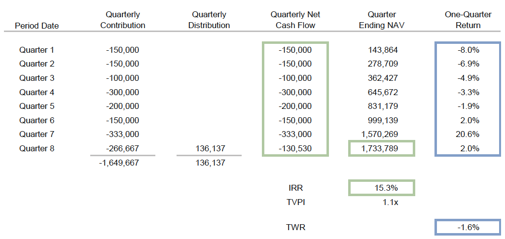
Source: Cambridge Associates LLC.
This divergence in returns is not confined to individual fund analysis. Use of the different methodologies can lead to very different results at the private investment portfolio level as well. In Figure 2, a private investment portfolio is compared to the CA benchmark universe using both measures (IRR and compounded TWR).
The top graph shows the portfolio’s performance against the relevant benchmark on an IRR basis over one- through ten-year time periods. In this comparison, the portfolio outperforms the benchmark in seven of the ten periods measured and outperforms over every period longer than three years. The bottom graph uses the same portfolio and benchmark universe, but employs the compounded TWR methodology to calculate returns. Using this calculation, the portfolio only outperforms in four of the ten periods. Notably, the largest difference occurs over the six-year time period: on an IRR basis, the portfolio outperforms by 1,165 basis points (bps); on a compounded TWR basis, the portfolio outperforms by only 201 bps. The results are also directionally inconsistent at times. Over ten years, the portfolio outperforms by 188 bps on an IRR basis but trails the benchmark by 60 bps using compounded TWRs! See “Convergence of TWRs and IRRs Is Not a Given” on page 6 for more on the use of IRRs versus TWRs.
Figure 2. The Disconnect Between IRRs and TWRs for a Private Investment Portfolio
Hypothetical Example
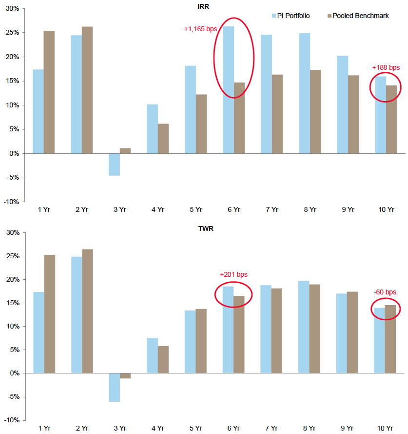
Source: Cambridge Associates LLC.
Convergence of TWRs and IRRs Is Not a Given
Many institutions use compounded TWRs to measure the performance of private investments to maintain consistent methodologies and compensation structures across the portfolio, and use the argument that compounded TWRs and IRRs should converge over time. This argument is flawed. Convergence can happen to the extent that a portfolio approaches “steady state”—that is, at least half of the portfolio is composed of mature funds and there are no meaningful strategy shifts or changes to the target allocation. At steady state, a program’s net cash flows are the same order of magnitude across periods (quarters). In this situation, because cash flows are in the same “range,” the TWR calculation’s independent handling of each quarter will not distort performance. Note, however, that even when compounded TWR and IRR results have converged, the introduction of extreme cash flows, which could happen in any number of scenarios such as a huge win in venture or meaningful increase or decrease in commitment pace, would immediately cause the results to diverge again. The longer the time horizon, the more severe such divergence can be. The graph below illustrates this point using the Cambridge Associates U.S. Venture Capital benchmark universe. This universe is a reasonable proxy for a steady-state portfolio because it comprises more than 900 funds across all stages of the fund lifecycle. The IRRs and compounded TWRs seem to demonstrate convergence until the tech bubble in 2000 and 2001. At that point, the methodologies diverge significantly: the IRRs continue to be impacted by large distributions received in the late 1990s, while the compounded TWRs are more heavily impacted by large scale declines in valuations when the bubble burst. Once the extreme event falls outside the considered time period, the two methodologies converge once again.
In addition to measuring portfolio performance by compounding TWRs, some institutions benchmark IRRs for private investments against public TWRs. As described in this paper, these calculations are fundamentally different: one considers size and relative timing of cash flows, while the other ignores this distinction by considering each period independently. Despite the popularity of benchmarks like S&P 500 plus 500 bps in investors’ policies on private benchmarking, using a benchmark like this is an apples-and-oranges comparison and is not appropriate. To more accurately measure private performance, investors should use IRRs to calculate private investment performance and compare those returns to a public market equivalent calculation.
U.S. Venture Capital Index Five-Year Rolling Periods
March 31, 1990 – June 30, 2010
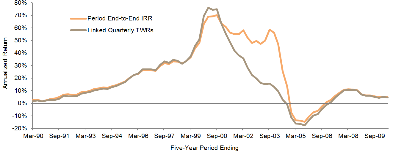
Source: Cambridge Associates LLC.
Limitations of IRRs. While we believe that IRRs are the most appropriate measure for private investments, the metric is by no means devoid of problems. Given that the IRR assumes that all distributions are reinvested at the same rate as the IRR itself, the performance of early commitments can have a disproportionate impact (good or bad) on since-inception performance. Early cash flows can “lock in” subsequent long-term returns, leading the IRR to overstate or understate the true level of a portfolio’s returns. For an investor that benefitted from strong venture capital distributions in the 1990s, for example, the IRR likely overstates the true level of returns, because subsequent investments are unlikely to have generated the same level of returns. In the hypothetical example in Figure 3, the entire portfolio can be written off with little impact on the IRR.
Figure 3. Early Performance Strongly Influences IRRs for a Fund: Example 1
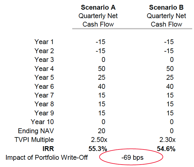
In this hypothetical example, the fund can be completely written off with a barely noticeable change in the fund’s IRR.
Source: Cambridge Associates LLC.
Note: Transactions occur at period-end for simplicity.
At the fund level, another issue for IRRs is that they can be “managed” given the right circumstances. Since IRRs are driven by the size and timing of cash flows, to the extent that a manager can create large distributions early in a fund’s life, a manager can “lock in” an overstated fund IRR. For example, trading-oriented distressed managers tend to have high IRRs and low cash-on-cash multiples. In the example in Figure 4, the fund generated meaningful distributions after only one year. These large distributions will likely be recycled into new opportunities, but have served to create an outsized IRR compared to the more modest multiple of invested capital.
Figure 4. Early Performance Strongly Influences IRRs for a Fund: Example 2
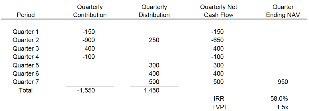
In this hypothetical example, a large early distribution leads to a high IRR but a low multiple.
Source: Cambridge Associates LLC.
To put IRRs in context, we recommend always reviewing IRRs alongside cash-on-cash multiples. Distributed to paid-in (DPI) and total value to paid-in (TVPI) multiples provide valuable insight into cash returns and cannot be “locked in” or managed like the IRR can. In addition, investors with established, mature portfolios whose since-inception returns are affected by this phenomenon may prefer to emphasize five- and ten-year returns that exclude prior periods of strong cash flows.
Understanding the differences in the TWR and IRR calculation methodologies and their limitations is critical to appropriately establish private investment benchmarking policies and to properly interpret private investment performance.
Incorporating Private Investments into the Total Portfolio Return. While we do not consider TWRs an adequate measure of private investment performance, in one area the use of quarterly TWRs is not only relevant, but necessary—the calculation of total portfolio (i.e., marketable and private investment) returns. In this context, the use of quarterly TWRs is acceptable because the private investment returns are not compounded across quarters to generate a TWR, but rather the quarterly private return is included as part of a weighted average quarterly return for the total portfolio. These combined quarterly portfolio returns can then be compounded across time periods to create a total portfolio return inclusive of both public and private investments.
The Importance of Time
The length of time over which investors measure performance is important. Return calculations for shorter periods place less emphasis on cash flows and are more sensitive to period-ending valuations. While accounting rules have changed to require mark-to-market valuations, managers use a variety of different methodologies in calculating fair value (some are much more conservative than others), leading to variability in ending valuations. Shorter time periods can also be greatly influenced by recent changes in commitment pace, a strategy shift, or extreme economic events. In the case of a mature, stable portfolio where commitments have been fairly constant over a long period of time and strategy implementation has remained fairly consistent, shorter time period returns, including those over one- and three-year periods, can offer some significance. However, in most cases, a five- or ten-year return gives a more accurate sense of performance.
When Do Returns Become Meaningful?
Understanding the length of time (and patience) required before any meaningful assessment of private investment performance can be made is a critical aspect of our benchmarking framework.
Many investors perform quantitative benchmarking analysis on funds and portfolios that we consider to be very young and for which such comparisons may be misleading. While there is widespread understanding of the J-curve (fund seasoning) among private investors, there is little definitive information about when returns for a fund actually become meaningful. We have completed an analysis showing that fund performance takes quite some time to become meaningful, a concept that underlies our benchmarking framework.
Given the variations in fund lifecycles and valuation methodologies, we analyzed more than 2,100 private investment funds raised between 1995 and 2005 to determine when fund returns begin to provide meaningful guidance as to a fund’s relative performance. While there’s some variation around the mid-1990s, our analysis shows that most funds require about six years before they “settle” into their ultimate quartile rankings as measured by IRR, and some strategies and vintages do not settle until sometime during year seven. On average, funds have settled into their ultimate quartiles between 5.8 years and 6.8 years into their lives (Figure 5).
Figure 5. Median Number of Years to Settle into Final Quartile Ranking
As of September 30, 2012 • Vintage Years 1995–2005
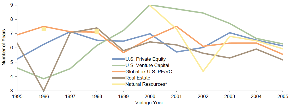
Source: Cambridge Associates LLC.
Notes: Graph shows the median age at which a fund settles into its final quartile ranking for each vintage year. The top and bottom 5% of each asset class are considered outliers and were excluded from the analysis.
*Vintage years 1995, 1997, and 1999 for natural resources have an insufficient number of funds in the sample to produce a meaningful analysis.
The argument could be made that if a fund tends to oscillate between two quartiles before ultimately settling sometime around year six of its life, then assessing relative performance may, in fact, be meaningful at an earlier point in time. However, our analysis shows that 80% to 90% of all funds in the sample were at one time ranked in three different quartiles during the course of their lifecycles and about 40% were ranked in each of the four quartiles at some point (Figure 6). In addition, 37% of the funds in our universe shifted quartiles between years six and seven of their lives, and 22% continued to shift between years eight and nine (Figure 7)!
Figure 6. Number of Quartile Rankings Experienced Throughout Fund Life
As of September 30, 2012 • Vintage Years 1995–2005
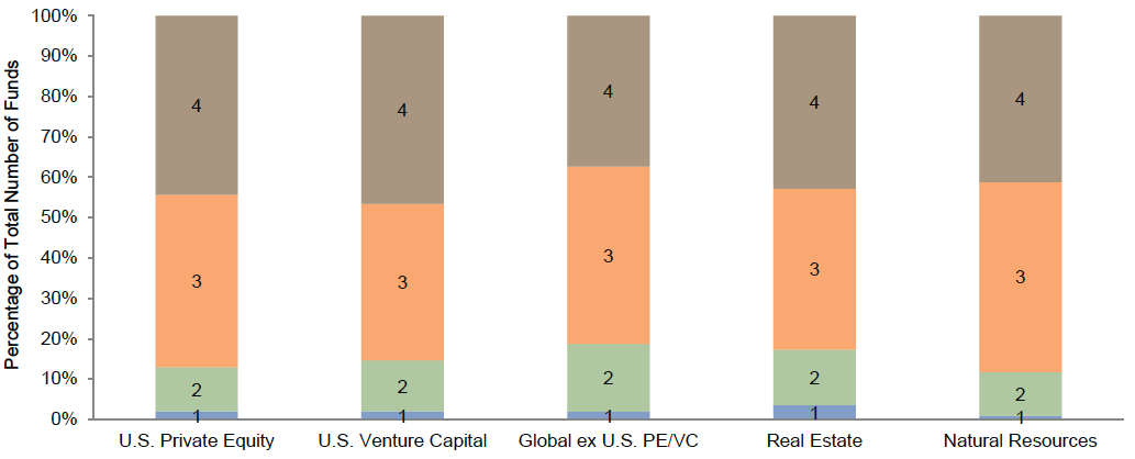
Source: Cambridge Associates LLC.
Notes: Graph shows the number of different quartile rankings each fund experienced throughout the life of the fund or as of September 30, 2012. Rankings are on a quarterly basis.
Based on this analysis, we believe that placing too much weight on a manager’s performance earlier than five to six years into a fund’s life cycle can lead to incorrect conclusions and poor selection of follow-on funds. Save for a big, obvious win or, conversely, a big, obvious loss, investors should pay little attention to any comparative benchmarking until an investment is at least five years old. In practice, this is a difficult exercise for investors and one that they understandably struggle with. In our view, early follow-on decisions should not be based on performance alone, but grounded in a thorough understanding of a manager’s organization, strategy, and ability to execute.
At the portfolio level, our analysis implies that investors should not attempt to derive much meaning from aggregate private portfolio returns and benchmark comparisons until the program is at least eight years old, assuming a steady commitment pace. Investors that ramp up commitments in the years following a portfolio’s inception should wait even longer. Ignoring returns for a meaningful portion of the portfolio is understandably difficult. To ensure insight into the performance of “seasoned” funds, investors could consider grouping the private investment portfolio into “mature” and “less mature” sub-portfolios for reporting purposes, with appropriate attention to performance and full benchmarking detail focused on the mature funds.
Figure 7. Quartile Movement by Fund Age
As of September 30, 2012 • Vintage Years 1995–2005
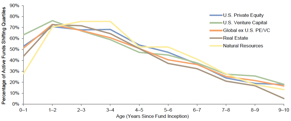
Source: Cambridge Associates LLC.
Notes: Graph shows the percentage of active funds that shifted quartile rankings for each year of the fund’s life. The top and bottom 5% of each asset class are considered outliers and were excluded from the analysis.
Framework for Benchmarking Private Investments
Having examined the best method to calculate private investment performance and the length of time for relative performance to become meaningful, we propose a framework for benchmarking private investment portfolios that looks broadly at these investments, assessing the degree of out/underperformance versus public alternatives, the investor’s manager selection skill, and the investor’s skill in selecting the right strategies at the right times. Investors employing the tools we suggest to evaluate each of these aspects of the investment will be able to answer the following three questions:
- Was the decision to allocate capital to privates a good one?
- Did we select good managers?
- Within our private investments, did we make good allocation decisions?
Performance vs. Public Markets
We believe that comparing private investment returns to public market alternatives is the best way to evaluate whether the decision to allocate capital to private investments was beneficial. Public market equivalent (PME) analysis provides an answer to the fundamental question: Was it worth taking on the illiquidity?
A PME represents a private investment—specifically private transactions—under public market conditions. Private investment contributions are invested “on paper” in a chosen public market index and distributions are taken out of the public index. Performance of this public equivalent can then be measured through using private investment metrics such as IRRs and multiples, and the results are then compared to the corresponding measures for the actual private investment to compute value add.
Some investors argue against the use of PME because it’s a mathematical construct and no investor would or could have invested in this way. While this is a legitimate concern, any methodology that is broadly applicable and properly accounts for the time value of money in the private investment cash flows requires some sort of construct. Certain approaches allow for private-to-public comparisons under specific conditions (e.g., what if private investment commitments had been funded from a bond allocation and proceeds reinvested in a public equity allocation), and while these are informative in proper context, they’re not broadly applicable.
Another consideration is the end-point sensitivity of this type of analysis. PME results can be heavily impacted by the state of the public markets over shorter periods of time. For example, few private investments will show outperformance in the current environment given the run-up in many public markets since 2009. The need to focus on longer periods of returns, as discussed earlier, pertains to PME analysis as well. Over the long term, these near-term dislocations between public and private valuations will have less impact on the analysis.
Which PME? We considered numerous PME and non-PME private-to-public comparison methodologies as part of our research. Each possesses slightly unique characteristics and exhibits varying degrees of robustness. They rank differently in terms of consistency, and conclusions about private investment value add (sign and magnitude) can vary across methodologies. Some of the most widely recognized methodologies include:
- Long-Nickels (simple PME): Actual private investment contributions are invested in public market index, and actual distributions are taken out.
- Strengths: This approach is common and intuitive.
- Considerations: When private investment distributions are high, public returns may not be strong enough to boost PME NAV to a level that can fund these distributions in the public equivalent, triggering the “negative NAV” problem that can, in turn, lead to unintuitive/non-meaningful results.
- Kaplan-and-Schoar (K&S) PME: A ratio of future values of private investment distributions and contributions, invested at the public index return. A ratio greater than one implies private investment outperformance. This approach is labeled “PME” but is not actually constructed by buying/selling public shares per the private investment cash flow schedule.
- Strengths: This approach is well known, intuitive, easy to explain, and avoids the pitfalls of the IRR calculation.
- Considerations: The ratio is not consistently indicative of the magnitude of value add.
In an effort to address the potential issues associated with existing methodologies, we developed a new measure, the Cambridge Associates Modified PME, or mPME. Like the Long-Nickels method, mPME assumes that private investment capital calls are used to purchase public shares, while private investment distributions represent the sale of those shares. However, under mPME, private investment contributions are invested in the public market index, and distributions are taken out in the same proportion as in the private investment. Specifically, with each distribution, mPME “sells” the same proportion of the dollar value of shares owned by the public equivalent as the private investment sells in private shares. 1
This methodology is robust. In contrast to other PME methodologies, mPME ensures that distributions from the public equivalent will—by design—never exceed what is available for distribution, avoiding the “negative NAV” problem. In addition, it allows for the calculation of DPI and TVPI multiples that can be compared to a private fund or portfolio. Comparing private investments to the public alternative on both an IRR and multiples basis gives investors a clear understanding of relative performance.
Some PME methods try to incorporate the impact of leverage on returns by making blanket assumptions about its use by managers. While true that leverage can be a significant component of private investment returns, the goal of the PME analysis is to determine if investors have been compensated for the illiquidity and administrative burden of private investments. As such, the leverage question does not play a role in this particular analysis.
Which Public Index? Role in portfolio should be the driving factor in selecting the appropriate public market index to use in mPME analysis. A simple approach would be to consider all private investments as growth drivers in the overall portfolio and lump them together versus a single public index that is based on the return objective for the allocation. A slightly more complicated approach would be to break out the portfolio into growth (VC/PE) and inflation hedging (some natural resources and real estate strategies) and assign different public indices for each. Arguably, either of these methods should provide a reasonable point of comparison to the public alternatives. The decision of whether to lump or split the portfolio into various benchmarks is unique to each investor and should be based on the role that private investments are perceived to serve within the larger portfolio.
Premium Over Publics. Another investor-specific decision is whether private investments should require a specified premium over public markets. Nearly all institutions invest in private investments due to their history of generating returns in excess of what is usually achieved in traditional, marketable asset classes. The trade-off for investing in privates is illiquidity and the added administrative burden of completing detailed subscription documents, managing the capital call and distribution cash flows, and dealing with a potentially more complicated audit process. An investor with a sufficiently liquid portfolio and large back office staff may determine that any premium over public markets is a good outcome for private investments. Another investor with a largely illiquid portfolio or with fewer administrative resources may require a premium over public indices to justify locking up additional capital. Typical premiums average 3% over public markets. At first glance, a premium of 3% may not sound like much. However, assuming a 6% real return on public investments over the long term, the resulting 9% required return on private investments is actually a 50% increase over the required return for publics!
Manager Selection
The second question in our benchmarking framework is: did we select good managers? Once an investment is mature enough to merit detailed benchmarking, we believe private investment medians and quartile rankings provide the best measure of whether a given investment was a good selection compared to other private funds raised in the same environment and that employ a similar strategy. Other metrics often used to gauge a fund’s relative performance such as the pooled return, which can be skewed by the larger funds in a benchmark, or the arithmetic mean, which is impacted by the dispersion of returns within the sample set, are less meaningful indicators.
The appropriate peer universe is specific to the role an investment plays in each investor’s portfolio. One investor may choose to benchmark a U.S. IT-focused venture fund raised in 2004 against other U.S. IT-focused venture funds raised in the same year, while another might benchmark that same fund against global venture funds (including all strategies) raised in 2004. The desire to evaluate a fund versus very closely related funds must be balanced against the need to maintain a minimum number of funds in the universe to return a statistically meaningful result. A minimum of 20 funds provides an ideal sample set, with five funds present in each quartile. A minimum of 12 funds is probably necessary to provide significant results in terms of quartile breakpoints. Investors mainly concerned with comparing to a median may consider a universe as small as eight funds meaningful.
While private-to-private benchmarks are the best gauge of manager selection skill, PME analysis can also be instructive. For this analysis, investors may compare manager performance to the most similar public index for each manager or each fund. For example, the Russell 2000® Index could be used for venture funds, the MSCI All Country World Index could be used for global large-cap buyout funds, and the NAREIT Industrial could be used for industrial-focused real estate funds.
Allocation Decisions
The third question in the framework is: within our private investments, did we make good allocation decisions? To examine the value added as a result of allocation decisions within private investments, we recommend creating custom-weighted pooled benchmarks. Investors can use this methodology to gauge the effectiveness of specific strategy and sub-strategy allocation and timing decisions. Suppose an institution had been investing in private equity since 1995 but didn’t allocate to venture until 2000. To conduct an analysis on allocation decisions, the investor would construct a benchmark based on the weights of the actual allocations of the portfolio and then compare that result with a second benchmark based on alternative allocation weightings. Comparing two benchmark scenarios allows investors to isolate the effectiveness of allocation decisions and quantify the value add without the impact of manager selection. This methodology can be used to gauge strategy, vintage year, and geographic allocation decisions.
There are two important methodological variables associated with this type of analysis—the type of data used in the analysis and the weighting methodology.
Custom-weighted benchmarks can be constructed using either the combined IRR method or pooled transaction method. The combined IRR method “calculates” a return from a series of IRRs (weighted average IRR), while the pooled transaction method pools the underlying transactions of the benchmark universe to create a stream of cash flows on which to calculate an IRR. The two approaches are completely different mathematically and intuitively and may or may not produce similar results. We believe that pooled transaction method is the correct way to create custom-weighted benchmarks.
The only way to calculate a true benchmark return for the purposes of assessing allocation choices is to construct a benchmark in the same manner that a portfolio is constructed. Combining the underlying cash transactions of the benchmark universe produces a composite stream of cash flows that is representative of real investment decisions and actual IRRs can be calculated from the results. While medians, arithmetic means, quartiles, minimums, and maximums all provide useful context to understand the performance of an individual fund, when considering any more elaborate composite (for example, multi-vintage year, multi-strategy portfolios, etc.), any mathematical combination of the underlying returns (IRRs) has little chance of producing a number that matches the true return had the portfolio been invested in the specified manner. Put differently, more elaborate composites created by combining IRRs are arbitrary numbers that may “feel” right, but are not reflective of what one could accomplish by “investing in the benchmark.”
The next question that naturally arises asks which weighting methodology should be applied to the cash flows—commitment, invested capital, or market value. The simplest answer is that weights should be determined by the decision that investors control—they only control the scale and timing of commitments. Invested capital and market value are dynamic measures over which investors have no control. Managers control these decisions and the intent of the allocation analysis is to eliminate the influence of manager selection. In addition, since both invested capital and market value will change over time, weighting by either of these measures would call for the ongoing “restatement” of weightings over time.
The results of this dynamic analysis may influence how investors think about portfolio construction and exposures, and could impact how the portfolio is invested going forward based on lessons learned from the past. While PME and private investment medians and quartiles are useful as defined benchmarks that are monitored from quarter to quarter for mature funds and portfolios, the allocation analysis described above is best reserved for periodic, in-depth portfolio reviews. Pooled custom benchmarks, weighted by investor commitments, allow investors to evaluate performance in a dynamic way and provide insights into longer-term trends—a static benchmark would not serve this purpose.
The Framework in Practice: A Case Study
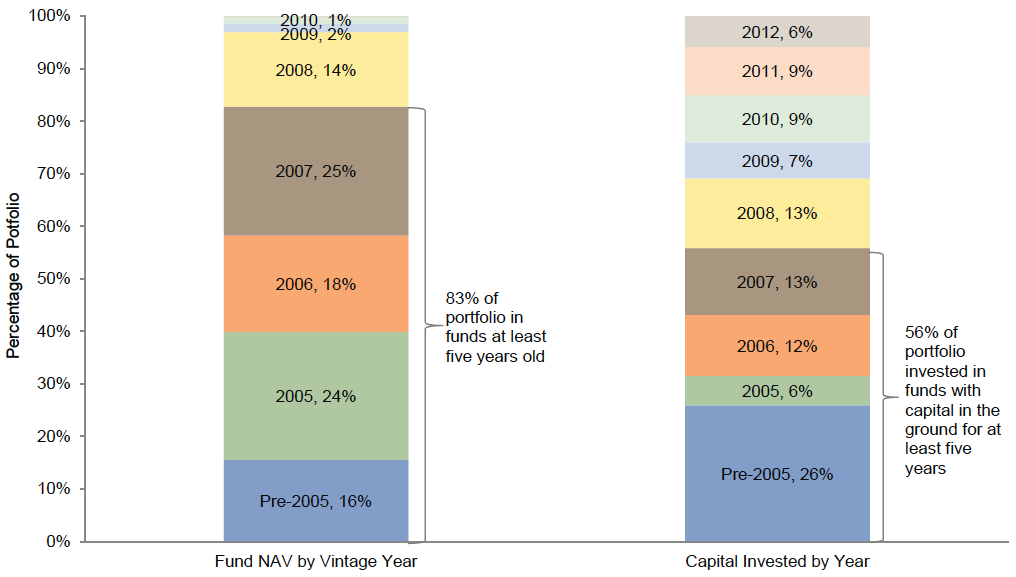
A complete review of private portfolio performance should always start with a review of the portfolio’s maturity. In this case study, over 80% of the portfolio is invested in funds that are at least five years old. However, a look-through to when the capital was actually invested reveals that less than 60% of the invested capital has been in the ground for at least five years (Figure 8). A portfolio can be considered mature if at least 40% of the invested capital has been in the ground for five years or more.
Figure 8. Case Study: Examination of Private Investment Portfolio Maturity
Source: Cambridge Associates LLC.
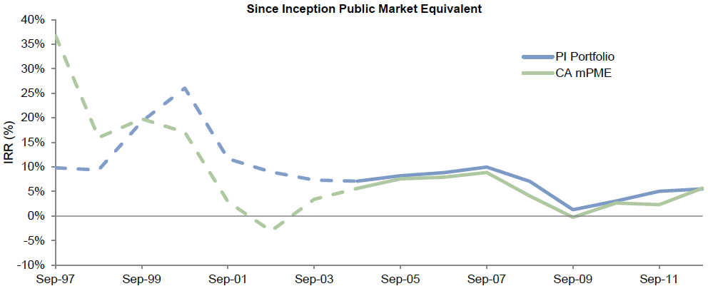
The next step in the analysis is to consider how additive the private investments have been as compared to the public market alternatives. Figure 9 demonstrates that once the sample portfolio began to mature around 2004, private investments have consistently added value over time. After narrowing from 2003 to 2007, the spread widened slightly in 2008 during the global financial crisis as public markets fell significantly more than private investments. In 2012, the spread narrows and inverts with publics outperforming as they recovered from the extreme losses suffered in the downturn.
Figure 9. Case Study: Did Allocating to Privates Add Value? Since Inception Analysis
Source: Cambridge Associates LLC.
Notes: Cambridge Associates Modified Public Market Equivalent (CA mPME) is composed of the following public indices: S&P 500, Russell 2500™, FTSE® NAREIT All Equity REITs, and S&P GSCI™ Energy. Dashed line prior to September 30, 2004, indicates that the portfolio is not mature yet and therefore analysis is not meaningful.
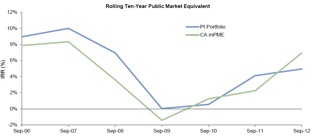
To smooth out the impact of extreme periods of performance, investors may prefer to review rolling five- or ten-year periods as we do in Figure 10. This also addresses the potential issue of an IRR that’s “locked-in” due to strong early cash flows.
Figure 10. Case Study: Did Allocating to Privates Add Value? Rolling Ten-Year Analysis
Source: Cambridge Associates LLC.
Notes: Cambridge Associates Modified Public Market Equivalent (CA mPME) is composed of the following public indices: S&P 500, Russell 2500™, FTSE® NAREIT All Equity REITs, and S&P GSCI™ Energy.
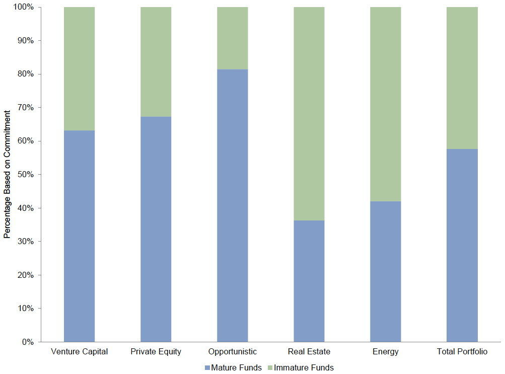
Evaluating manager selection is the second part of the framework. Again, investors will first want to understand the investments’ maturity to determine whether the benchmark comparisons are meaningful. For this case study, Figure 11 details the breakout of mature versus immature commitments by strategy. Looking just at the mature funds, we analyze both the quartile placement by capital invested (Figure 12) and quartile ranking by strategy (Figure 13). In this example, 55% of the mature portfolio has been invested with funds that have outperformed the median fund in the benchmark. Looking at quartiles by asset class of mature funds, the investor has done a good job selecting energy managers and has done less well in the venture capital space.
Figure 11. Case Study: Did Manager Selection Add Value? Maturity Analysis
Mature vs. Immature Funds
Source: Cambridge Associates LLC.
Figure 12. Case Study: Did Manager Selection Add Value? Performance of Mature Funds
Mature Portfolio by Quartile (Based on Invested Capital)
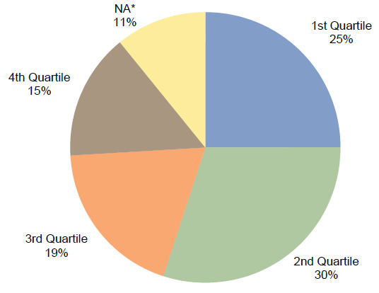
Source: Cambridge Associates LLC.
*Funds unable to be ranked due to a limited sample size.
Figure 13. Case Study: Did Manager Selection Add Value? Quartile Rankings of Mature Funds by Strategy
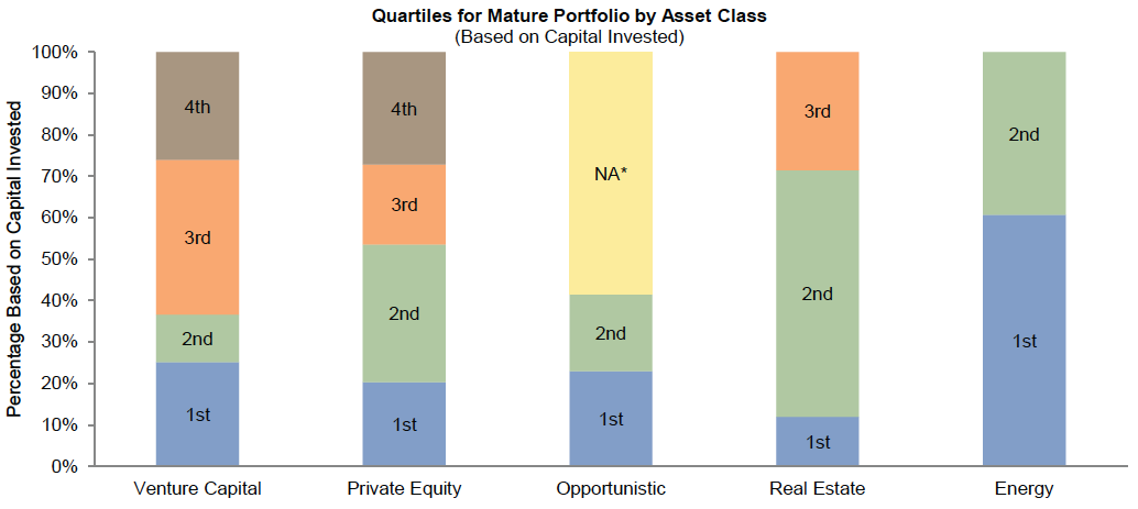
Source: Cambridge Associates LLC.
*Funds unable to be ranked due to a limited sample size.
The final part of the framework aims to measure allocation decision attribution. This analysis does not apply a standard benchmark, but instead seeks to answer portfolio-specific “what if” questions by comparing two benchmark scenarios. For this particular portfolio, the investor could examine the following decisions (among others):
- All of the energy exposure has been through private equity–style managers. What if historical commitments to the sector had been split between energy private equity managers and upstream & royalties managers?
- A portfolio of 100% energy private equity (based on the investor’s commitment pace and sizing) outperforms a similar portfolio of 75% energy private equity/25% energy upstream & royalties by 20 bps. Therefore, the decision to only invest in private equity–style managers was additive.
- What if the institution had invested its heavily U.S.-focused buyouts portfolio more globally since the start?
- A buyouts portfolio of 70% United States, 20% Europe, and 10% Asia and Rest of World outperforms the investor’s actual geographic allocation by approximately 70 bps. Therefore, the investor would have benefited from geographic diversification.
- The investor’s venture portfolio is heavily weighted toward IT and diversified venture funds. Would the institution have benefitted from doing more health care–focused venture funds?
- The investor’s decision to focus only on IT and diversified focused funds resulted in approximately 100 bps of outperformance. Therefore, the decision to avoid health care–focused strategies was additive.
Conclusion
Measuring and benchmarking private investment performance is an ambiguous and complex process. The lack of a single “right” measure leads to inconsistency across the industry and makes it difficult to decompose the various drivers of performance. Our framework seeks to solve that problem by identifying the key performance questions to address and then measuring success across a series of key metrics using a set of tools that can be applied in a consistent manner.
While the framework provides answers to the key questions, investors should wait until their portfolios are sufficiently seasoned before deriving any meaning from the results. The possibility of strong returns drives investors toward private investments, but those investors must go into privates with a clear understanding of the patience required to measure and realize these returns. In many cases, the ultimate payout from private investments is realized long after staff and investment committees have turned over. Understanding the potential for this asset class and embracing the reality that returns are not meaningful for quite some time, and therefore investment decisions should not be based on early returns, is a crucial element for success.
Footnotes
Jill Shaw - Jill Shaw is a Partner for the Endowment & Foundation Practice at Cambridge Associates.
About Cambridge Associates
Cambridge Associates is a global investment firm with 50+ years of institutional investing experience. The firm aims to help pension plans, endowments & foundations, healthcare systems, and private clients achieve their investment goals and maximize their impact on the world. Cambridge Associates delivers a range of services, including outsourced CIO, non-discretionary portfolio management, staff extension and alternative asset class mandates. Contact us today.